ai
How diffusion models generate images: the math, the architecture, the samplers
A diffusion model does not "draw" an image — it learns to reverse a process that turns an image into noise, then walks that reverse path from pure noise back to a picture. This is the full engineering tour: the DDPM objective, score matching and the SDE/ODE view, the U-Net-to-DiT architecture shift, the samplers that make it fast, and the conditioning stack that makes it obey a prompt.
AI-generated draft · reviewed and editedThis text was generated with AI as a first draft, then reviewed and edited by the author, who holds editorial responsibility for it.

How diffusion models generate images: the math, the architecture, the samplers
A diffusion model does not draw. It reverses a destruction. Take a real image, add a little Gaussian noise, repeat a thousand times, and the picture dissolves into pure static. A diffusion model learns the inverse: given a noisy image and a step number, predict how to remove a little noise. To generate, you start from pure noise and walk that reverse path back to a picture. That single idea — learn the reverse of a noise-adding Markov chain — is the engine behind Stable Diffusion, DALL·E, Midjourney, FLUX, and most of the image models shipping today.
This article is the full engineering tour, grounded in the primary sources. We cover the mathematics (the DDPM objective, score matching, and the SDE/ODE unification), the architectures (U-Net → Latent Diffusion → Diffusion Transformers → MMDiT), the samplers that turn a thousand-step chain into a ten-step one (DDIM, classifier-free guidance, DPM-Solver, EDM), and the conditioning stack that makes a model obey a text prompt (CLIP/T5, cross-attention, ControlNet, LoRA). Every equation and number below is quoted from the cited paper.
[video: Reversing the Noise — Mohammed Kmail]
The forward process: destroying an image with noise
The starting point is the Denoising Diffusion Probabilistic Model (DDPM) of Ho, Jain and Abbeel (2020). A diffusion model is a latent-variable model whose latents have the same dimensionality as the data. The forward process (also called the diffusion process) is a fixed Markov chain that gradually adds Gaussian noise to the data according to a variance schedule β_1, …, β_T:
q(x_1:T | x_0) = ∏_{t=1}^{T} q(x_t | x_{t-1}), q(x_t | x_{t-1}) = N(x_t; √(1-β_t) x_{t-1}, β_t I) (Eq. 2)Each step scales the previous image down by √(1-β_t) and adds Gaussian noise of variance β_t. The paper notes the crucial property that this admits sampling x_t at an arbitrary timestep in closed form. With α_t := 1-β_t and ᾱ_t := ∏_{s=1}^{t} α_s:
q(x_t | x_0) = N(x_t; √ᾱ_t x_0, (1-ᾱ_t) I) (Eq. 4)This is the workhorse equation of training. Because the marginal is closed-form, you never have to simulate the whole chain to get a noisy sample at step t — you take a clean image x_0, scale it by √ᾱ_t, and add noise of variance 1-ᾱ_t. As t grows, ᾱ_t shrinks toward zero and the image is progressively destroyed. The DDPM paper uses a linear schedule of β_t from β_1 = 10⁻⁴ to β_T = 0.02 over T = 1000 steps.
The reverse process: learning to denoise
The reverse process is a Markov chain with learned Gaussian transitions, starting from pure noise p(x_T) = N(x_T; 0, I):
p_θ(x_0:T) := p(x_T) ∏_{t=1}^{T} p_θ(x_{t-1} | x_t), p_θ(x_{t-1} | x_t) := N(x_{t-1}; μ_θ(x_t, t), Σ_θ(x_t, t)) (Eq. 1)The paper explains why Gaussian conditionals suffice: "When the diffusion consists of small amounts of Gaussian noise, it is sufficient to set the sampling chain transitions to conditional Gaussians too, allowing for a particularly simple neural network parameterization." Training optimizes the variational bound on negative log-likelihood (the ELBO):
E[-log p_θ(x_0)] ≤ E_q[-log p_θ(x_0:T) / q(x_1:T | x_0)] =: L (Eq. 3)The bound decomposes into a sum of KL divergences between the forward-process posterior and the learned reverse transitions. The key simplification comes from reparameterizing the model to predict the noise ε rather than the mean. The paper shows that with the ε-prediction parameterization, the per-step loss simplifies to a plain mean-squared error between the true noise and the model's prediction:
L_simple := E_{x_0, ε} [ || ε - ε_θ(√ᾱ_t x_0 + √(1-ᾱ_t) ε, t) ||² ] (Eq. 14, simplified)This is the entire training loop. Sample a random timestep t, sample Gaussian noise ε, corrupt the image to x_t, and train the network to recover ε from x_t and t. The paper's Algorithm 1 is exactly: sample t ~ Uniform({1,…,T}), sample ε ~ N(0, I), then take a gradient step on ∇_θ ||ε - ε_θ(√ᾱ_t x_0 + √(1-ᾱ_t) ε, t)||².
The paper frames this as a primary contribution: "a certain parameterization of diffusion models reveals an equivalence with denoising score matching over multiple noise levels during training and with annealed Langevin dynamics during sampling." On unconditional CIFAR-10, DDPM achieved an Inception score of 9.46 and a state-of-the-art FID of 3.17 — the first time a diffusion model matched GANs without adversarial training.
The score-matching view: learning the gradient of the data density
The DDPM paper explicitly connects to score-based generative models. Song and Ermon (2019) introduced the idea of generating samples via Langevin dynamics using gradients of the data distribution estimated with score matching. The score is the gradient of the log-density, ∇_x log p(x) — a vector field pointing toward regions of high probability. Their key insight: "Because gradients can be ill-defined and hard to estimate when the data resides on low-dimensional manifolds, we perturb the data with different levels of Gaussian noise, and jointly estimate the corresponding scores." This is the Noise-Conditional Score Network (NCSN), and sampling uses annealed Langevin dynamics — "we use gradients corresponding to gradually decreasing noise levels as the sampling process gets closer to the data manifold."
The connection is deep: predicting the noise ε in DDPM is mathematically equivalent to estimating the score of the perturbed data distribution. The noise the model predicts points in the direction of the score, scaled. This is why the DDPM loss "resembles denoising score matching over multiple noise scales indexed by t."
The unification: diffusion as a stochastic differential equation
Song, Sohl-Dickstein, Kingma, Kumar, Ermon and Poole (2021) unified both families under one framework. Their paper, "Score-Based Generative Modeling through Stochastic Differential Equations," shows that both DDPM and score matching are discretizations of the same continuous-time process. The forward process is an SDE that "smoothly transforms a complex data distribution to a known prior distribution by slowly injecting noise," and there is a corresponding reverse-time SDE that "transforms the prior distribution back into the data distribution by slowly removing the noise." Crucially: "the reverse-time SDE depends only on the time-dependent gradient field (aka, score) of the perturbed data distribution."
The paper also derives an equivalent probability flow ODE — a deterministic ordinary differential equation that "samples from the same distribution as the SDE, but additionally enables exact likelihood computation, and improved sampling efficiency." This ODE is the theoretical foundation of the fast samplers we use today. The paper introduced a predictor-corrector framework and achieved record-breaking CIFAR-10 results: Inception score 9.89, FID 2.20, and "high fidelity generation of 1024×1024 images for the first time from a score-based generative model."
The architecture: from U-Net to Diffusion Transformers
The network that predicts the noise is the heart of the system, and it has gone through two generations. The DDPM paper introduced the U-Net backbone — a convolutional encoder-decoder with skip connections, inherited from PixelCNN++ with a few changes. The DiT paper describes it precisely: "The model is convolutional, comprised primarily of ResNet blocks," with "additional spatial self-attention blocks... interspersed at lower resolutions." The time step t is injected via a sinusoidal positional embedding, and the model is conditioned on it through adaptive normalization layers.
Nichol and Dhariwal (2021) improved the recipe in "Improved Denoising Diffusion Probabilistic Models," introducing a cosine noise schedule (which the SD3 paper later adopted) and learning the reverse-process variance Σ_θ instead of fixing it — both of which materially improved sample quality and log-likelihood.
Latent Diffusion: the move that made it practical
The single most consequential architectural decision was Rombach, Blattmann, Lorenz, Esser and Ommer's (2022) Latent Diffusion Model (LDM) — the basis of Stable Diffusion. The problem with pixel-space diffusion is cost: "optimization of powerful DMs often consumes hundreds of GPU days and inference is expensive due to sequential evaluations." The paper cites 150–1000 V100 days to train the most powerful pixel-space models, and "producing 50k samples takes approximately 5 days on a single A100 GPU."
The fix: run the diffusion process in the latent space of a pretrained autoencoder instead of pixel space. The paper's framing: "we apply them in the latent space of powerful pretrained autoencoders." The encoder downsamples the image by a factor f, and the paper investigates f ∈ {1, 2, 4, 8, 16, 32}. Their finding: "LDM-4 and -8 offer the best conditions for achieving high-quality synthesis results" — a 4× or 8× downsampling factor. This is why Stable Diffusion runs on a 64×64 latent for a 512×512 image: the diffusion model works in a space 64× smaller, then a VAE decoder upscales the latent back to pixels. The paper reports that LDMs "significantly reduc[e] computational requirements compared to pixel-based DMs."
The LDM paper also introduced the cross-attention conditioning mechanism: "By introducing cross-attention layers into the model architecture, we turn diffusion models into powerful and flexible generators for general conditioning inputs such as text or bounding boxes." This is the mechanism that lets a text prompt steer generation — the text tokens attend into the U-Net's spatial features at every resolution.
Diffusion Transformers: the scaling-law shift
Peebles and Xie (2023) showed the U-Net inductive bias is not essential. Their Diffusion Transformer (DiT) replaces the U-Net with a transformer operating on latent patches: "We train latent diffusion models of images, replacing the commonly-used U-Net backbone with a transformer that operates on latent patches." The paper's central finding is a clean scaling law: "DiTs with higher Gflops—through increased transformer depth/width or increased number of input tokens—consistently have lower FID."
For conditioning, DiT found that adaptive layer norm (adaLN-Zero) works best among the variants tested (adaptive layer norm, cross-attention, and extra input tokens). Their largest model, DiT-XL/2, achieved a state-of-the-art FID of 2.27 on class-conditional ImageNet 256×256, with a high-capacity backbone of 118.6 Gflops. This established the pattern that modern image models follow: transformers scale predictably with compute.
MMDiT and rectified flow: the modern backbone
The current generation — Stable Diffusion 3 and FLUX — builds on Esser et al.'s (2024) MMDiT (multimodal DiT) and rectified flow. The paper, "Scaling Rectified Flow Transformers for High-Resolution Image Synthesis," makes two moves. First, it replaces the diffusion forward process with rectified flow, which "connects data and noise in a straight line" — a straight path that "could be simulated with a single step and is less prone to error accumulation," unlike curved paths that "require many integration steps." Second, it introduces an architecture with "separate weights for the two modalities and enables a bidirectional flow of information between image and text tokens, improving text comprehension, typography, and human preference ratings."
The paper demonstrates "a predictable scaling trend in the validation loss" and shows "a lower validation loss correlates strongly with improved text-to-image synthesis." This is the architecture behind the highest-quality open text-to-image models shipping today.
Sampling: turning 1000 steps into 10
Training is one thing; generation is another. A naive DDPM needs all T = 1000 reverse steps, each a full network evaluation. The entire field of fast sampling exists to cut that number, and it rests on the probability flow ODE from the SDE paper: sampling is solving an ODE numerically, and better solvers mean fewer steps.
DDIM: deterministic, non-Markovian, 10–50× faster
Song, Meng and Ermon (2021) introduced Denoising Diffusion Implicit Models (DDIM). The insight: DDPM's generative process is "the reverse of a particular Markovian diffusion process," but you can generalize to "a class of non-Markovian diffusion processes that lead to the same training objective." These "can correspond to generative processes that are deterministic, giving rise to implicit models that produce high quality samples much faster." The headline result: "DDIMs can produce high quality samples 10× to 50× faster in terms of wall-clock time compared to DDPMs." Because the process is deterministic, DDIM also enables "semantically meaningful image interpolation directly in the latent space" — a property that makes latent-space editing possible.
Classifier-free guidance: the knob that controls fidelity
The single most important sampling technique for text-to-image is classifier-free guidance (CFG) from Ho and Salimans (2022). The idea: "we jointly train a conditional and an unconditional diffusion model, and we combine the resulting conditional and unconditional score estimates to attain a trade-off between sample quality and diversity." In practice, the model is trained to predict the noise both with and without the conditioning (the conditioning is randomly dropped during training), and at sampling time the two estimates are combined with a guidance weight w:
ε_guided = ε_θ(x_t, t) + w · (ε_θ(x_t, t, c) - ε_θ(x_t, t))Higher w pushes the sample harder toward the conditioning — sharper adherence to the prompt, but less diversity and a risk of oversaturation. Lower w gives more variety but weaker prompt adherence. This is the "guidance scale" you see in every image-generation UI, and it is the direct descendant of the classifier-guidance tradeoff the paper describes: "trade off mode coverage and sample fidelity."
DPM-Solver and EDM: high-order ODE solvers
Lu, Zhou, Bao, Chen, Li and Zhu (2022) pushed sampling to 10–20 function evaluations with DPM-Solver. Their key contribution is an "exact formulation of the solution of diffusion ODEs" that "analytically computes the linear part of the solution, rather than leaving all terms to black-box ODE solvers." The result: "DPM-Solver can generate high-quality samples in only 10 to 20 function evaluations on various datasets," achieving 4.70 FID in 10 function evaluations and 2.87 FID in 20 on CIFAR-10, a 4–16× speedup over prior training-free samplers.
Karras, Aittala, Aila and Laine (2022) took a different, more empirical route in "Elucidating the Design Space of Diffusion-Based Generative Models" (EDM). They argued the field was "unnecessarily convoluted" and "present a design space that clearly separates the concrete design choices" — the noise schedule, the preconditioning of the score network, and the sampler. Their improvements yielded "new state-of-the-art FID of 1.79 for CIFAR-10 in a class-conditional setting and 1.97 in an unconditional setting, with much faster sampling (35 network evaluations per image)." The EDM framework is the basis of the k-diffusion samplers used across the ecosystem.
Conditioning: how a prompt steers the noise
A diffusion model that only denoises produces random images. To make it obey a prompt, you condition it. The text is first encoded into a vector by a pretrained text encoder, then injected into the network. Stable Diffusion uses the CLIP text encoder (Radford et al., 2021), which was trained on 400 million (image, text) pairs to predict which caption goes with which image — a representation that "enables zero-shot transfer of the model to downstream tasks." Modern models like SD3 and FLUX additionally use a T5 text encoder (Raffel et al., 2020) for stronger language understanding. The text tokens are injected into the U-Net via the cross-attention layers introduced in the LDM paper.
ControlNet: spatial control without retraining
Text alone cannot specify pose, depth, or edges. Zhang, Rao and Agrawala (2023) introduced ControlNet, which "locks the production-ready large diffusion models, and reuses their deep and robust encoding layers pretrained with billions of images as a strong backbone to learn a diverse set of conditional controls." The mechanism is elegant: a trainable copy of the network is added, connected via "zero convolutions (zero-initialized convolution layers) that progressively grow the parameters from zero and ensure that no harmful noise could affect the finetuning." Because the base model is frozen, ControlNet can be trained on small datasets ("< 50k") and adds spatial conditions like "edges, depth, segmentation, human pose" without touching the base weights.
LoRA: cheap fine-tuning via low-rank updates
Full fine-tuning of a diffusion model is expensive. LoRA (Low-Rank Adaptation) from Hu et al. (2021) sidesteps this by freezing the base weights and learning only low-rank update matrices. The paper's premise: "As we pre-train larger models, full fine-tuning, which retrains all model parameters, becomes less feasible." LoRA constrains the weight update to a low-rank factorization, so the number of trainable parameters is a fraction of the full model. In the diffusion ecosystem, LoRA is the standard way to teach a model a new style, a new character, or a new concept — the Hugging Face diffusers library explicitly supports "loading and using adapters like LoRA."
The practical stack: diffusers and the model family
The de facto open-source toolchain is Hugging Face's diffusers library, which "is a library of state-of-the-art pretrained diffusion models for generating videos, images, and audio." Its core abstraction is the DiffusionPipeline, "an API designed for easy inference with only a few lines of code" and "flexibility to mix-and-match pipeline components (models, schedulers)." This modularity is the practical payoff of the theory: the model (U-Net or DiT), the scheduler (DDIM, DPM-Solver, EDM), and the conditioning (text encoder, ControlNet, LoRA) are all swappable components. The Stable Diffusion family spans SD 1.5, SDXL, and SD3 (the latter built on the MMDiT/rectified-flow architecture), with FLUX as the leading open alternative.
The bottom line
A diffusion model is a score estimator wearing a denoiser's hat. It learns the reverse of a noise-adding process, and generation is numerically solving the reverse SDE/ODE from pure noise. The engineering that made it practical is a chain of clean ideas: the closed-form forward marginal (DDPM), the score-matching equivalence, the probability flow ODE, the latent-space move (LDM), the transformer scaling law (DiT), the straight-line flow (rectified flow), the fast ODE solvers (DDIM, DPM-Solver, EDM), and the conditioning stack (cross-attention, CFG, ControlNet, LoRA). Each one is a small, verifiable contribution — and together they turned a 1000-step Markov chain into the image generators we use every day.
Sources
- DDPM — "Denoising Diffusion Probabilistic Models," Ho, Jain, Abbeel, 2020, arXiv:2006.11239 — https://arxiv.org/abs/2006.11239 (equations 1–4, 14; Algorithm 1; CIFAR-10 IS 9.46 / FID 3.17)
- Score matching — "Generative Modeling by Estimating Gradients of the Data Distribution," Song & Ermon, 2019, arXiv:1907.05600 — https://arxiv.org/abs/1907.05600 (NCSN, annealed Langevin, CIFAR-10 IS 8.87)
- SDE/ODE unification — "Score-Based Generative Modeling through Stochastic Differential Equations," Song, Sohl-Dickstein, Kingma, Kumar, Ermon, Poole, 2021, arXiv:2011.13456 — https://arxiv.org/abs/2011.13456 (reverse-time SDE, probability flow ODE, CIFAR-10 IS 9.89 / FID 2.20, 1024×1024)
- Improved DDPM — "Improved Denoising Diffusion Probabilistic Models," Nichol & Dhariwal, 2021, arXiv:2102.09672 — https://arxiv.org/abs/2102.09672 (cosine schedule, learned variance)
- Latent Diffusion / Stable Diffusion — "High-Resolution Image Synthesis with Latent Diffusion Models," Rombach, Blattmann, Lorenz, Esser, Ommer, 2022, arXiv:2112.10752 — https://arxiv.org/abs/2112.10752 (latent space, downsampling f∈{1,2,4,8,16,32}, LDM-4/-8 best, cross-attention, 150–1000 V100 days)
- DiT — "Scalable Diffusion Models with Transformers," Peebles & Xie, 2023, arXiv:2212.09748 — https://arxiv.org/abs/2212.09748 (U-Net→transformer, adaLN-Zero, Gflops scaling, DiT-XL/2 FID 2.27, 118.6 Gflops)
- SD3 / MMDiT / rectified flow — "Scaling Rectified Flow Transformers for High-Resolution Image Synthesis," Esser et al., 2024, arXiv:2403.03206 — https://arxiv.org/abs/2403.03206 (rectified flow straight-line paths, separate modality weights, bidirectional text-image flow)
- DDIM — "Denoising Diffusion Implicit Models," Song, Meng, Ermon, 2021, arXiv:2010.02502 — https://arxiv.org/abs/2010.02502 (non-Markovian, deterministic, 10–50× faster, latent interpolation)
- Classifier-free guidance — "Classifier-Free Diffusion Guidance," Ho & Salimans, 2022, arXiv:2207.12598 — https://arxiv.org/abs/2207.12598 (joint conditional/unconditional training, quality-diversity tradeoff)
- DPM-Solver — "DPM-Solver: A Fast ODE Solver for Diffusion Probabilistic Model Sampling in Around 10 Steps," Lu, Zhou, Bao, Chen, Li, Zhu, 2022, arXiv:2206.00927 — https://arxiv.org/abs/2206.00927 (10–20 function evaluations, 4.70 FID@10 / 2.87 FID@20 on CIFAR-10, 4–16× speedup)
- EDM — "Elucidating the Design Space of Diffusion-Based Generative Models," Karras, Aittala, Aila, Laine, 2022, arXiv:2206.00364 — https://arxiv.org/abs/2206.00364 (design space, FID 1.79 class-cond / 1.97 uncond CIFAR-10, 35 network evaluations)
- CLIP — "Learning Transferable Visual Models From Natural Language Supervision," Radford et al., 2021, arXiv:2103.00020 — https://arxiv.org/abs/2103.00020 (400M image-text pairs, zero-shot transfer)
- ControlNet — "Adding Conditional Control to Text-to-Image Diffusion Models," Zhang, Rao, Agrawala, 2023, arXiv:2302.05543 — https://arxiv.org/abs/2302.05543 (zero convolutions, frozen backbone, edges/depth/segmentation/pose)
- LoRA — "LoRA: Low-Rank Adaptation of Large Language Models," Hu et al., 2021, arXiv:2106.09685 — https://arxiv.org/abs/2106.09685 (low-rank weight updates)
- diffusers — Hugging Face diffusers library — https://huggingface.co/docs/diffusers (DiffusionPipeline, mix-and-match models/schedulers, LoRA adapters)
keep reading

The Model That Would Not Speak: System One AI on Your Own Machine
One support ticket, three decision models, no graphics card: I ran 144M, 421M and 4.2B System One models on my own CPU and wrote down what each one said. The 144M model missed "I am cancelling on Friday"; the vague ticket produced three different answers. What a decision model is, how to run one with llama.cpp or Ollama, and how Kev, Nimble, Laya and Jev compare.
ai · 19 min · 2026-10-14
Mistral Large 4: The Cybersecurity Model That Refuses to Refuse
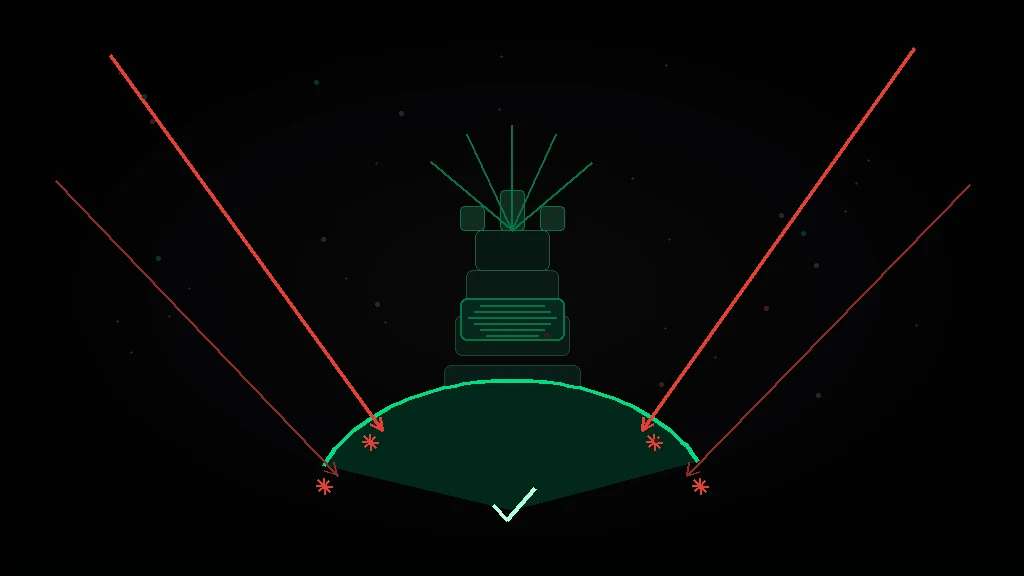
Six frontier models refuse ≥98% of real CVE reproduce-and-patch tasks. Mistral Large 4 completes them — and gets 82% right, the highest score ever measured. Charts, independent failure data, and the honest anatomy of what a defender’s model can and cannot do.
ai · 18 min · 2026-10-07

How to Become an AI Expert: The Path That Actually Produces One
Anthropic’s own postings say the quiet part: formal certifications are explicitly optional, and the screening question asks whether you have shipped an LLM system to production for real users. The full path: what the market actually hires for, the seven-layer builder’s stack, the learning science on why watching fails, the honest failure numbers — and a build ladder to start this month.
ai · 21 min · 2026-10-05